Table of content:
Training one robot leg
This section gives some example and draws some conclusions about the training of a single robot leg.
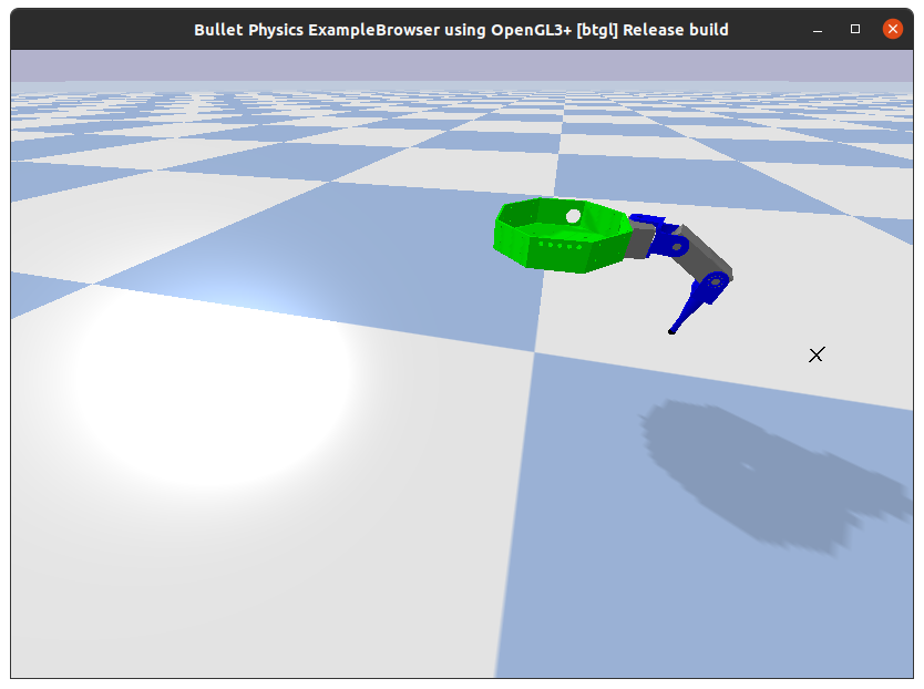
The environment resets the leg to a random position. The agent has to command each servomotors to move the fingertip to a random objective (visualized by the cross).
# Reset all joint using normal distribution
for j in self.joint_list:
    p.resetJointState(self.robot_id, j,
                      np.random.uniform(low=-np.pi/4, high=np.pi/4))

# Set random target in a 3D box
self.target_position = np.array([
    np.random.uniform(0.219 - 0.069*self.delta, 0.219 + 0.069*self.delta),
    np.random.uniform(0.020 - 0.153*self.delta, 0.020 + 0.153*self.delta),
    np.random.uniform(0.128 - 0.072*self.delta, 0.128 + 0.072*self.delta),
])
Note
Some early tests were done on StableBaselines3 but as the library is currently being developed, the training was failing and the average episode reward was constant.
First tests with a fixed objective
With pytorch-a2c-ppo-acktr-gail
The defaults hyperparameters given in the pytorch-a2c-ppo-acktr-gail README are recommanded and are able to give good results for a first training.
Warning
The reward function is only using the distance to a fixed objective. This agent learned only to go to a fixed target.
The observation vector used here is:
| Num | Observation |
|---|---|
| 0 | position (first joint) |
| 1 | velocity (first joint) |
| 2 | torque (first joint) |
| 3 | position (second joint) |
| 4 | velocity (second joint) |
| 5 | torque (second joint) |
| 6 | position (third joint) |
| 7 | velocity (third joint) |
| 8 | torque (third joint) |
| 9 | the x-axis component of the fingertip position |
| 10 | the y-axis component of the fingertip position |
| 11 | the z-axis component of the fingertip position |
The reward is -target_distance,
target_distance being the distance between the fingertip and the target.
Note
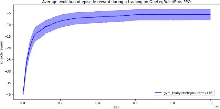
16 trainings with different seeds were averaged to plot the previous figure. The light blue zone corresponds to the standard error.
The training is successful and converges after 300k steps.
The enjoy.py script shows the leg moving to the fixed target,
but it vibrates after reaching the objective.
With StableBaselines
Start StableBaselines Docker as explained in previous page. Then in Jupyter web interface,
check_env.ipynbwill check that OpenAI Gym environments are working as expected,one_leg_training.ipynbis an example of PPO training on one leg,render.ipynbwill render the agent to a MP4 video or a GIF.
As planned, it works as well as pytorch-a2c-ppo-acktr-gail on PyTorch,
but this time we get much more tools such as
TensorBoard data and graph.
As StableBaselines stands out as being an easy PPO implementation with a clear documentation and hyperparameters, all the following training were done with it.
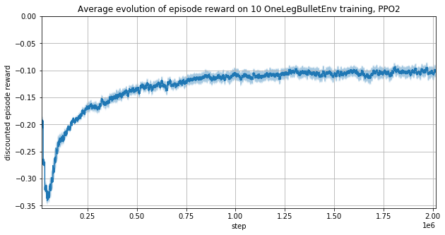
Learning to go to a random target
Now we fix delta = 0.5 to pick the target (x, y, z) such as,
0.1845 ≤ x ≤ 0.2535,
-0.0565 ≤ y ≤ 0.0965,
0.0920 ≤ z ≤ 0.164.
Batch size
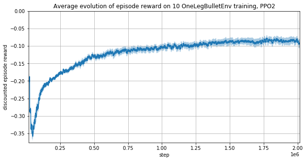
As the target changes at each episode start, the batch size need to be large enough to make sure it contains some variance.
First tests
We used the following code and hyperparameters to train using StableBaselines:
from stable_baselines.common.policies import MlpPolicy
from stable_baselines.common import set_global_seeds
from stable_baselines import PPO2
from stable_baselines.common.vec_env import SubprocVecEnv
import gym
from gym.wrappers import TimeLimit


def make_env(rank, seed=0):
    """
    Init an environment

    :param rank: (int) index of the subprocess
    :param seed: (int) the inital seed for RNG
    """
    timestep_limit = 128

    def _init():
        env = gym.make("gym_kraby:OneLegBulletEnv-v0")
        env = TimeLimit(env, timestep_limit)
        env.seed(seed + rank)
        return env
    set_global_seeds(seed)
    return _init

seed = 1
num_cpu = 16
env = SubprocVecEnv([make_env(i, seed) for i in range(num_cpu)])

# Use `tensorboard --logdir notebooks/stablebaselines/tensorboard_log/doc1` to inspect learning
model = PPO2(
    policy=MlpPolicy,
    env=env,
    gamma=0.99,  # Discount factor
    n_steps=512,  # batchsize = n_steps * n_envs
    ent_coef=0.0,  # Entropy coefficient for the loss calculation
    learning_rate=2.5e-4,
    lam=0.95,  # Factor for trade-off of bias vs variance for Generalized Advantage Estimator
    nminibatches=32,  # Number of training minibatches per update.
                      # For recurrent policies, the nb of env run in parallel should be a multiple of it.
    noptepochs=4,  # Number of epoch when optimizing the surrogate
    cliprange=0.2,  # Clipping parameter, this clipping depends on the reward scaling
    verbose=False,
    tensorboard_log="./tensorboard_log/doc1/",

    seed=seed,  # Fixed seed
    n_cpu_tf_sess=1,  # force deterministic results
)
model.learn(total_timesteps=int(2e6))
The observation vector used here is:
| Num | Observation |
|---|---|
| 0 | position (first joint) |
| 1 | velocity (first joint) |
| 2 | torque (first joint) |
| 3 | position (second joint) |
| 4 | velocity (second joint) |
| 5 | torque (second joint) |
| 6 | position (third joint) |
| 7 | velocity (third joint) |
| 8 | torque (third joint) |
| 9 | the x-axis component of the fingertip position |
| 10 | the y-axis component of the fingertip position |
| 11 | the z-axis component of the fingertip position |
| 12 | the x-axis component of the target |
| 13 | the y-axis component of the target |
| 14 | the z-axis component of the target |
The reward is -target_distance,
target_distance being the distance between the fingertip and the target.
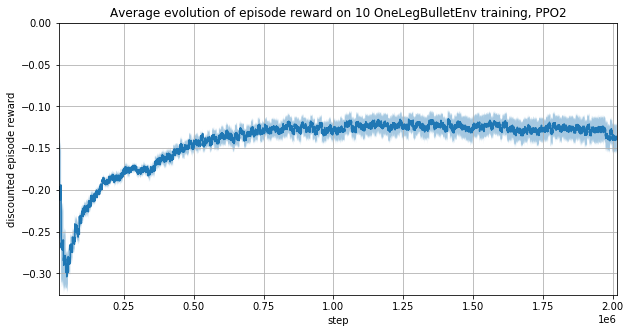
Removing motors torque from observations
The observation vector used here is:
| Num | Observation |
|---|---|
| 0 | position (first joint) |
| 1 | velocity (first joint) |
| 2 | position (second joint) |
| 3 | velocity (second joint) |
| 4 | position (third joint) |
| 5 | velocity (third joint) |
| 6 | the x-axis component of the fingertip position |
| 7 | the y-axis component of the fingertip position |
| 8 | the z-axis component of the fingertip position |
| 9 | the x-axis component of the target |
| 10 | the y-axis component of the target |
| 11 | the z-axis component of the target |
The reward is -target_distance,
target_distance being the distance between the fingertip and the target.
It seems that the training is a bit faster without motors torques as the observation vector is smaller.
The leg does not always reach the target and vibrates.
Using cosinus and sinus of motor positions
This idea comes from OpenAI Gym Reacher-v2 environment.
The observation vector used here is:
| Num | Observation |
|---|---|
| 0 | cos(position) (first joint) |
| 1 | sin(position) (first joint) |
| 2 | velocity (first joint) |
| 3 | cos(position) (second joint) |
| 4 | sin(position) (second joint) |
| 5 | velocity (second joint) |
| 6 | cos(position) (third joint) |
| 7 | sin(position) (third joint) |
| 8 | velocity (third joint) |
| 9 | the x-axis component of the fingertip position |
| 10 | the y-axis component of the fingertip position |
| 11 | the z-axis component of the fingertip position |
| 12 | the x-axis component of the target |
| 13 | the y-axis component of the target |
| 14 | the z-axis component of the target |
The training using cosinus and sinus is slower.
Using the vector from the target to the fingertip
This idea also comes from OpenAI Gym Reacher-v2 environment.
The observation vector used here is:
| Num | Observation |
|---|---|
| 0 | position (first joint) |
| 1 | velocity (first joint) |
| 2 | position (second joint) |
| 3 | velocity (second joint) |
| 4 | position (third joint) |
| 5 | velocity (third joint) |
| 6 | the x-axis component of the vector from the target to the fingertip |
| 7 | the y-axis component of the vector from the target to the fingertip |
| 8 | the z-axis component of the vector from the target to the fingertip |
| 9 | the x-axis component of the target |
| 10 | the y-axis component of the target |
| 11 | the z-axis component of the target |
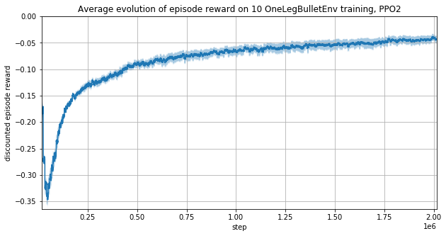
Putting the vector from the target to the fingertip rather than the fingertip position results in better learning performances.
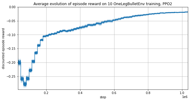
Optimizing hyperparameters
The observation used here is the same as the previous section but the hyperparameters are now:
num_cpu=32
ent_coef=0.01
nminibatches=64
noptepochs=30
total_timesteps=1e6
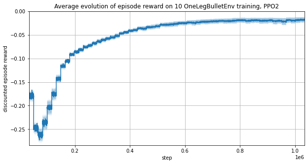
Increasing noptepochs increases GPU usage and make the learning converge much faster.
A learning of 1 million steps is done under 8 minutes on a Nvidia GTX1060 and an Intel i7-8750H.
Training without fingertip position
All previous learning put the fingertip position in the observation vector. This is problematic to transfer from simulation to reality as this vector cannot be measured on the real system. It may be found by solving the dynamic of the robot leg. Another approach is to remove this data from the observation and see how much the learning performance fall.
The observation vector used here is:
| Num | Observation |
|---|---|
| 0 | position (first joint) |
| 1 | velocity (first joint) |
| 2 | position (second joint) |
| 3 | velocity (second joint) |
| 4 | position (third joint) |
| 5 | velocity (third joint) |
| 6 | the x-axis component of the target |
| 7 | the y-axis component of the target |
| 8 | the z-axis component of the target |
Not only the policy learned to reach the target but it did it with less variance between learning runs.